| Back |
|---|
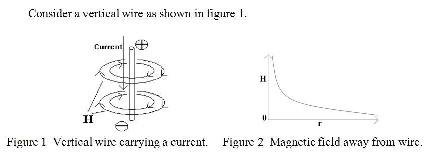
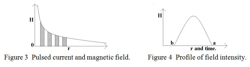
Assuming that the current flows from the positive end of the wire to the negative end, (i.e. downwards in the diagram), the direction of the resultant magnetic field is as shown. (Maxwell’s Cork Screw Rule). For a constant current, the magnetic field falls off with distance, r, from the centre of the wire as 1/r as shown in figure 2. For a uniform distribution of current across the cross-section of the wire, although the magnetic field completely surrounds the wire, it does not enter it. As the current is turned on the magnetic field can be visualised as spreading out from the wire at the speed of light. If, instead of a steady current, pulses of current are sent through the wire, pulses of magnetic field radiate from the wire and a “snapshot” of the magnetic field distribution at an instant of time might look like figure 3.
Each current pulse produces a cylinder or ring of magnetic field around the wire and each ring expands outwards with time into the surrounding space. Now consider that the current pulses are not rectangular but “half sine-wave” shaped so that each magnetic ring has a magnetic field profile as shown in figure 4. (Note that although “r” increases from left to right, time increases from right to left. I.e. the “switch-on” at “a” occurs before the “switch off” at “b”). Now, according to Maxwell’s equations, an electric field is produced by a changing magnetic field at right angles to it and at right angles to the direction of propagation, and a magnetic field is produced by a changing electric field with similar restrictions. The strength of either induced field is proportional to the rate of change of the other field. Let us examine in some detail the “sense” or “phase” of the induced electric field.
This is easily seen by reference to a toroid as frequently used as a mains transformer, where the iron core takes the place of the ring of magnetic field. A cross section of a toroid with a winding is depicted in figure 5. The usual conventions for field towards, , and away from, , the observer are used.
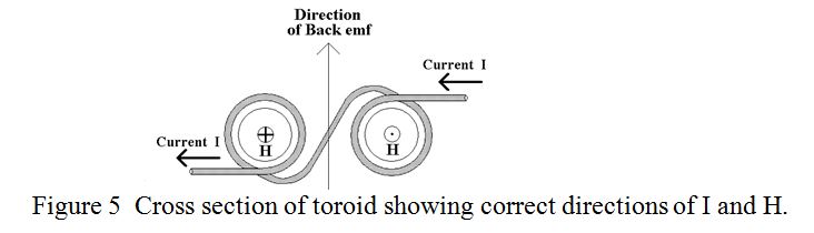
When the current, shown from right to left in the figure, and therefore the magnetic field is increasing, a “back-emf” is produced which tends to oppose the direction of the current, and this is shown by the single arrow through the middle of the toroid. In actual fact, electric field lines in space, (like magnetic field lines), do not terminate but form continuous loops. So the upward field lines through the centre of the toroid curl round and become downward field lines outside the toroid and re-join the upward lines through the centre of the toroid.
When the current and therefore the magnetic field is decreasing, the back-emf is in the opposite, downward, direction in the centre and upward outside the toroid. (This form of transformer, with a single turn secondary winding through the centre of the toroid, is frequently used in SWR meters to sample the transmission line current). The purpose of this rather detailed discussion is that it establishes the relationship between the directions of magnetic field, its direction of change, (i.e. increasing or decreasing) and the direction and sense of the induced electric field. Now let us apply this to the magnetic field resulting from the “half sine wave” current pulse in the wire. Examining the simplified case of the fields resulting from an isolated half sine wave is justified, since a real wave train is just a succession of half sine waves of alternate polarity.
Just as in the case of the toroid, the increasing magnetic field towards the observer induces an electric field around it, upwards behind it and downwards in front of it as depicted in figure 6.
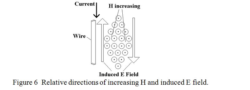
The E field surrounds the H field just as the H field surrounds the current. The upward directed E-field shown adjacent to the wire is responsible for the back-emf in the wire tending to oppose the rising current in the wire, and the downward directed E-field shown ahead of the H-field is what, (when it changes), will be responsible for the next induced H-field, and so on ad infinitum. It is this ability of each field to generate the other field ahead of it which gives E-M waves the ability to travel through a vacuum. Now let us consider the relative phases of the E and H fields.
Continue with the valid assumption of a “half sine wave” pulse of current and therefore of magnetic field. As described above, the induced E-field is produced outside the ring of magnetic field surrounding the vertical wire. (Consider the two dimensional case where the axes are the direction of propagation and the amplitude of the E or H fields) as shown in figure 7.
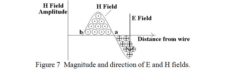
Although the E-field is produced outside the region of the H field, the maximum E-field is produced when the H field is changing at its fastest, i.e. as it crosses over from a decreasing “towards” field to an increasing “away from” field, shown as point “a”. So far we have dealt with an isolated current pulse and an isolated magnetic “half sine wave”. The argument is in no way invalidated if a succession of half sine waves of alternate polarity were generated. In this case the E-field to the right of point “a” generated by the decreasing H-field would have to fit in between the H-field half sine wave “a-b” and the next H-field half sine wave to its right, and its peak amplitude would be half way between its nulls as indicated in the figure.
Assuming that a sine wave H-field generates a sine wave E-field, then, extrapolating back from the E field negative peak to the abscissa, it is seen that the outgoing E-field is in phase with the outgoing H-field. Thus, an observer standing at the vertical wire and looking outward in the direction of propagation would see the instantaneous outgoing E and H fields as shown in figures 8a or 8b. (This is convenient for remembering because it can be made to fit the usual convention of using a cross to indicate an “away from” flow).
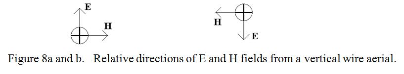
Thus, the E-field and H-field of an E-M wave are in temporal phase with each other but in spatial quadrature with each other and with the direction of propagation and in directions indicated by figures 8a nd 8b.
It is appreciated that the above note is more of an analogy than an explanation, which it is hoped will help the reader build a conceptual model. But like much in electro-magnetic wave theory it leaves several questions unanswered.
John, G0NVZ or Praeceptor?
| Back |
|---|