AB INITIO
| Back |
|---|
This article is written in response to a request to say a little more about what happens to the electrons in a klystron and a magnetron. The klystron amplifier and a kindred device, the Travelling Wave Tube were covered in simplified form last month. This month we take another look at the Magnetron.
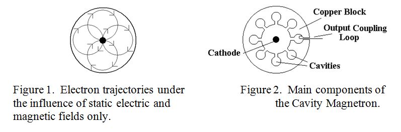
The workings of a Magnetron are more complicated than those of a klystron. As previously explained, the Magnetron is a “Crossed Field Device”. i.e. it needs both an electric and a magnetic field at right angles to make it work. The electric field is provided by a high tension supply of usually from one to twenty thousand volts, (depending on the required output power), applied between its central cathode and its surrounding cylindrical anode. It is this voltage which gives energy to the electrons and accelerates them from the cathode towards the anode. The magnetic field, (usually supplied by a permanent magnet), is applied parallel to the axis of the cathode and anode. A static magnetic field cannot give energy to electrons but it can deflect or accelerate them in a direction perpendicular to both the magnetic field and to their original direction of travel. If cavities were not machined into the anode, the electron trajectories under typical operating conditions would be as shown in figure 1, i.e. no anode current would flow because the magnetic field would “cut off” the anode current. As a reminder of what the inside of a cavity magnetron looks like, it is depicted in figure 2 which shows the main components.
With the magnetic field cutting off the anode current, all the electrons would return to the cathode with the same energy, (speed), as they left it. However, when microwave cavities are machined into the solid copper anode, electrons passing near the entrances of the cavities induce an electric field in the cavities which resonate at a frequency determined by the dimensions of the cavity. Thus, some electron gives up some of their kinetic energy to the cavity in the form of radio frequency energy. In so doing these electrons slow down, and instead of skimming past the open end of the cavity, they are pulled by the electric field onto one of the anode segments. Hence anode current flows. However, other electrons may either be in luck and similarly give up their energy to the RF field, or they may be out of luck and arrive a half cycle later when the RF field is in a direction to further accelerate them. Whereupon, they speeds up and may even return to the cathode with more energy than when they left it. If an electron returns with sufficient energy it may result in “secondary emission” from the cathode, thus releasing one or more electrons to go into the circulating cloud. You might think that this is a self balancing system with as many electrons giving energy to the RF field as extracting it, but this is not so. Electrons which have given energy to the RF field are removed from the system as anode current. Those which have extracted energy from the RF field live to fight another day and may even produce more electrons. The complicated orbits which individual electrons may take and the phyisics of electromagnetic wave formation inside the cavity magnetron has been described as “amongst the most complicated areas of classical physics, both from theorectical and practical viewpoints” When the magnetron is oscillating, the bunched electron cloud is eventually shepherded into “spokes” as in a wheel, the spokes of which rotate at a rate of two cavities per RF cycle. One of the advantages of the electron “spoke” sweeping past several resonant cavities is that the cavities modify the electron distribution in each spoke as it passes into something like a sine wave distribution as did the intermediate cavities of the multi-cavity Klystron. Otherwise the distribution of electrons in the bunch would be rich in harmonics as we saw in the two cavity klystron.
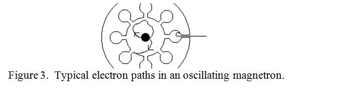
Two typical trajectories of individual electrons are depicted in figure 3, the upper one showing the path of an electron which passes cavities with an accelerating field, and the lower one showing the effect of passing cavities with a retarding field.
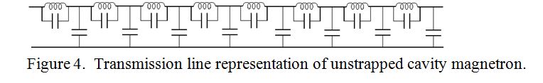
The original magnetron of Randall and Boot had 6 resonant cavities, but modern magnetrons usually have more, up to 20. More cavities means a bigger anode block which can handle more power, but the cavities interact, allowing the magnetron to operate in other than the desirable “Pi” mode. In the Pi mode, adjacent segments between cavities are 1800 out of phase. All modes however result in a whole number of cycles around the whole structure. The resonant frequency is mainly determined by the dimensions of the cavities but is slightly modified by the capacitance of each segment to the cathode and by the mutual coupling between adjacent cavities. The whole structure may be likened to a transmission line comprising parallel tuned circuits in series with intervening capacitors to earth as shown in figure 4.
“Strapping”, as discussed in the previous article, ensures that oscillation is only possible in the desirable “Pi mode”, but there are cheaper ways of manufacturing the anode block to achieve this end. One of these is to insert higher resonant frequency cavities, (at which frequency the magnetron does not produce output power), between the main cavities. This type is known as a “Rising Sun” magnetron, and an impression of one is shown in figure 5. This is probably the commonest type manufactured today.

The cathode and its electron emitting coating has to be of robust construction to withstand the high electrostatic stress of several thousand volts per millimetre at the cathode and a current of many amps without having its emissive coating stripped off together with the electrons. The humble microwave oven for cooking “fast food” is probably the main application of the cavity magnetron today.
PRAECEPTOR
| Back |
|---|